General relativity simulator | Ivan Goethals homepage

Simulating an orbit around a spherical mass

The curvature of space-time around a spherical mass is described by the Schwarzschild metric.

$c^2 d\tau^2 = \left(1 - \frac{2GM}{c^2 r} \right) c^2 dt^2 - \left(1 - \frac{2GM}{c^2 r} \right)^{-1} dr^2 - r^2 \left(d \theta^2 + sin^2 \theta d \varphi^2 \right)$
We provide an Excel file simulating the orbit of a test particle around the spherical mass using a straightforward forward Euler simulation.

Download link: 20161106_geodesic_line_simulation_riemann_schwarzschild_2d_v3
The simulation is performed in a 2-dimensional space where $\theta = \pi/2$ and $c=1$ meaning the metric reduces to:

$d\tau^2 = \left(1 - \frac{2GM}{r}\right) dt^2 - \left(1 - \frac{2GM}{r}\right)^{-1} dr^2 - r^2 d \varphi^2$
or

$d\tau^2 = \left[ \begin{matrix} dr & d \varphi & dt \end{matrix} \right] \left[ \begin{matrix} - \left(1 - \frac{2GM}{r}\right)^{-1} & 0 & 0 \\ 0 & - r^2 & 0 \\ 0 & 0 & \left(1 - \frac{2GM}{r}\right) \end{matrix} \right] \left[ \begin{matrix} dr \\ d \varphi \\ dt \end{matrix} \right] = g_{ij} dx^i dx^j$
where the right hand side uses Einstein notation.

Given coördinates $r, \varphi, t$ and first order derivatives $dr, d\varphi, dt$ at time $t=0$ , the 2nd order derivatives feeding the simulation can be derived using the geodesic equation:

$\frac{d^2x^{\mu}}{dq^2} + \Gamma^{\mu}_{\nu\lambda} \frac{dx^{\nu}}{dq} \frac{dx^{\lambda}}{dq} = 0$
where $\Gamma$ is derived from

$\Gamma^m_{ij} = \frac{1}{2}g^{ml} \left( \frac{\delta g_{il}}{\delta x^j} + \frac{\delta g_{lj}}{\delta x^i} - \frac{\delta g_{ji}}{\delta x^l} \right)$
again using Einstein notation and with $g^{ml}$ the inverse matrix of the metric $g$ .
The exact matrices $\Gamma$ are provided in the Excel.

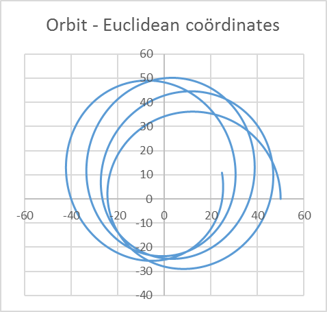
An example is provided below and can be simulated in the Excel by setting the starting values to $r = 50, \varphi = 0, t = 0$ and $\frac{dr}{d\tau} = 0, \frac{d\varphi}{d\tau} = 0.0024$ and the simulation step size to $d\tau=0.4$ .

Simulation with G=M=1, at a distance of about 25 times the Schwarzschild radius. Perihelium-shift is clearly visible.